
Principal Component Analysis (PCA) is a useful technique when you want to get a better understanding of a dataset containing a large number of correlated features. For example, in image processing, PCA is used for data compression. The main objective is to reduce the complexity of the data with a minimum loss of information.
In this post, we will first have look at PCA from a geometric approach to get an intuition how it works. Secondly, we will have the math behind PCA covered and see how its mathematical terminology translates to the statistical world. Finally, we will put this all together in an example, showing the most common output of a PCA analysis. You can find the data and the Jupyter notebook I created for generating the plots and calculations presented in this post here.
PCA: intuition
As an example, let’s consider this dataset containing the length and the width of 5 different classical cars:
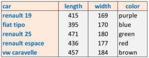
Clearly, both features are related to the overall non-measured characteristic “size” of the car. How can we map the two measured features “length” and “width” to the single feature “size”? In other words, how can we reduce the dimensionality of the data from 2 dimensions to just 1 dimension?
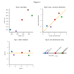
A graphical approach to answer this question looks as follows. First we plot the 5 cars in a two dimensional space (figure 1A). The length and the width of the cars are clearly correlated. This makes sense: big cars tend to be both longer and wider than small cars. Next, we draw a line in the direction of the highest variance of the data points (figure 1B). We rotate the plot to make this line coincide with the x-axis (figure 1C). Finally, we project the data points onto the x-axis (figure 1D). The result is an ordering of the cars along just 1 dimension, or in statistical parlance: along the first principal component direction.
PCA: math
The key question to answer now is: how do we find the orange dotted line in figure 1B? Let x be a p-dimensional vector containing the features of a specific sample. Two vectors a and b are orthogonal if and only if their dot product equals 0: a’b = 0. Therefore, the orthogonal projection λw of x onto w should satisfy the following equation:
(1) 
If we solve this equation for λ, we get the point on the vector w closest to the point x:
(2) 
Each of the vectors x, w and proj_w x has been visualized in figure 2.
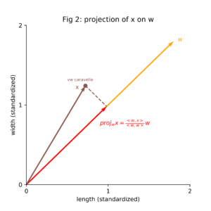
As the important thing about w is its direction (not its length), we can assume without loss of generality w to be the unit vector:
(3) 
Let X be a column wise mean-centered n x p feature matrix containing all n samples, i.e. x is any of the rows of X. The variance of the projected data as a function of w equals to:
(4) 
This scalar quantity is the so called quadratic form of X. It reflects the amount of variance in matrix X of the coordinate space defined by the vector w. We want to maximize this variance subject to w being a unit vector:
(5) 
We can solve this constrained optimization problem using the method of Lagrange multipliers:
(6) 
(7) 
(8) 
From this, we see that the vector w that maximizes Q(w) equals the eigenvector corresponding to the largest eigenvalue of ΣΣ:
(9) 
If we store all eigenvectors of ΣΣ in a p x p matrix W, we have:
(10) 
where ΛΛ is a diagonal matrix containing the eigenvalues corresponding to the eigenvector columns in W. As the columns of W form an orthogonal basis for the row and column space of ΣΣ, we have:
(11) 
and
(12) 
This equation reflects the eigen decomposition of matrix ΣΣ. Basically, it separates the row and column space into directions (as reflected by the columns of W) and magnitudes (as reflected by the diagonal elements of ΛΛ). The principal component directions of the data set X are the columns of W and can be found by performing this eigen decomposition on ΣΣ, the covariance matrix of X. It is common practice to sort the columns in W based on the magnitude of the diagonal elements in ΣΣ. The first column of W points in the direction of the highest variance of the projected data. The second column of W points in the second largest variance direction subject to the condition that this column in perpendicular to the first column, etc.
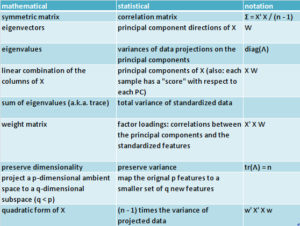
Terminology
When people talk about PCA, I see them using a mixture of mathematical and statistical terminology. This table gives a summary of the most common terminology from both perspectives.
Cars example
In this example we consider 24 classical cars, measured on 6 features each: engine displacement, power, speed, weight, length and width. The objective is to reduce the number of features without losing too much information.
First we calculate the correlation matrix of the data:
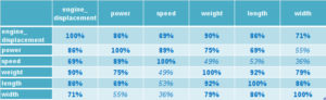
We see that the features are highly correlated, as we would expect. Larger cars tend to be more powerful. Except for the correlation between speed and size related features (weight, length and width) and power to width, all p-values are significant at the 0.5% level. Performing the eigen decomposition on this correlation matrix, as described in the section above, results in the eigenvalues and eigenvectors. The eigenvalues are often summarized in a so called scree plot, as shown in figure 3.
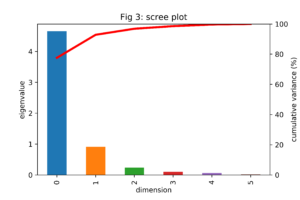
From this scree plot we learn that the first principal component explains close to 80% of the variation of the data. This percentage increases to more than 90% if we also include the second principal component. Note that the bars add up to 6, the total variance of the standardized data.
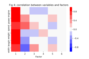
The factor loadings are the correlations between the eigenvectors and the standardized features from the data set, shown in figure 4. According to this heatmap, all features have a strong positive correlation with the first principal component while only power en speed have a strong positive correlation with the second principal component. Based on these observations, we might decide to label the first PC as “overall size” and the second PC as “relative power”.
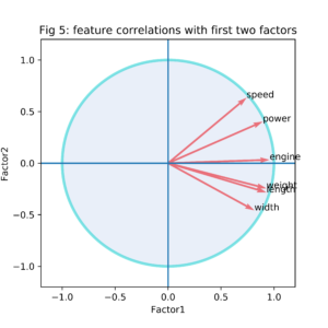
Another representation of the factor loadings related to the first two PC’s only is shown in figure 5. As correlations are always between -1 and 1, all vectors in this representation fall within the unit circle.
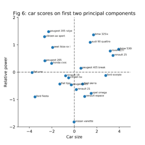
Figure 6 shows the original samples (24 cars) plotted in the two dimensions (PC1, PC2) space. The large powerful cars are located in the upper right corner of the plot. The small but powerful cars are located in the upper left corner of the plot. In comparison to the other cars, the Nissan Vanette is a medium sized car with a weak engine.
Conclusion
In this post we had a look at PCA from several perspectives. From a geometric perspective, PCA finds a projection of the data containing the highest amount of energy (variation). From a mathematical perspective, PCA entails an eigen decomposition on the correlation matrix. From a statistical perspective, PCA aims at finding the optimal trade-off between a reduced number of dimensions on one hand, and a minimum loss of information with respect to the standardized data on the other hand. In summary, PCA can be a powerful tool for getting a better understanding of high dimensional data, especially when we keep the following in mind:
- PCA makes the hidden assumption that principal components explaining a high percentage of the variance are more important than features explaining less variance. Although this assumption seems reasonable, it may not always be the case. From neuroscientist Mike X Cohen, I learned that in his field, variance is almost never the same as relevance, which is why PCA tends not to be useful for neural data. In short: “PCA assumes that variance equals relevance.”
- The outcomes of a PCA analyses are not scale invariant. Before performing the PCA we need to standardize each feature by subtracting the mean and dividing by the standard deviation.
- Labeling the principal components can be a tricky job; it is more an art than a science. If interpretation of the remaining features is a requirement, PCA can still be a useful tool for Exploratory Data Analysis, but not for communicating the final results.
Acknowledgements: I would like to express my gratitude to Mike X Cohen, neuroscientist, writer and teacher, for his valuable comments on this post.