
Last year, Tony Stenning explained on Blackrock Blog why it makes sense to introduce retirement plans for babies. In this post, I will discuss this interesting idea from an actuarial perspective. First I will provide some social background on the current global pension situation. Next, I will perform an analysis giving insight into the benefits and expenses of lifetime retirement savings. Finally, I will reserve the last part of this post for readers interested in the R code I used to perform the calculations and visualizations.
The next crisis
Ten years after the subprime mortgage crisis, many experts predict real estate prices are rising toward a new housing bubble. However, it is likely that bankrupt pension systems in the United States and Europe will turn out to be the trigger for the next collapse. According to the Hoover institute Essay Hidden Debt, Hidden Deficits, the unfunded obligations of the pension system sponsored by state and local governments in the United States continue to grow. With a market value funding ratio of less than 50%, unfunded accrued liabilities in the United States alone amount to a staggering $4 trillion. As a matter of fact, pension systems in several countries in the world are not sustainable and need major reform to prevent them from collapsing.
Retirement planning at birth
The idea to start retirement savings at birth, gives rise to the following two questions:
- what are the benefits of retirement savings starting at birth, compared to current practice where people do not start saving for their pension until they receive their first pay check?
- what would be the government expenses of the proposed system, compared to the current Social Welfare Pay-As-You-Go system?
Benefits
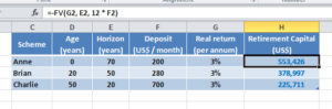
In order to understand how different time horizons effect pension benefits, we will compare the saving schemes for three individuals, each one investing a total amount of $168,000:
- Anne: deposits $200 per month from age 0 till 70 (=70 years)
- Brian: deposits $280 per month from age 20 till 70 (=50 years)
- Charlie: deposits $700 per month from age 50 till 70 (=20 years)
The results are summarized in the four following charts:
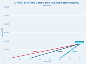
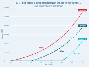
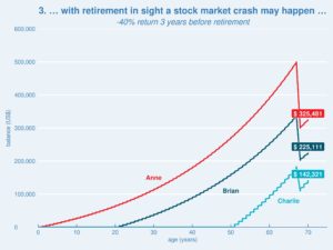
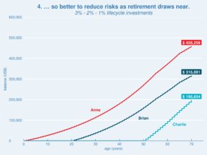
The charts clearly show the benefit of a longer investment horizon: in spite of their total amounts invested being equal to $ 168,000 (Chart #1), Anne will end up with a 46% higher retirement benefit than Brian and even 145% higher than Charlie (Chart #2). However, a stock market crash just three years before retirement will hit Anne the most (Chart #3). On the other hand, a longer investment horizon leaves more time for risk reduction without losing too much upside potential (Chart #4).
How do the pension capitals, presented in the charts above, compare to the current pension situation in the United States? According to an analysis from the Economic Policy Institute nearly half of all working-age US families have zero retirement account savings. The benefit an average retiree receives amounts to US$ 13,000 from the Social Welfare system plus a similar amount from additional pension schemes (DB-plans, 401(k), etc.). At the age of 70, these two benefits together represent a pension capital of about $250,000, significantly less than the capital accumulated by Anne in Chart #4.
Expenses
The current population of the United States of America is 327 million (and counting) with around 90% of the population younger than 70 years. Expenses for introducing Anne’s scheme next year would amount to $706 billion (=90% x 327 million x 12 x $200), around 4% of GDP. This is significantly less than the current public expenditure on old-age and survivors cash benefits, amounting to around 7% of GDP.
Implementation in MS Excel and R
The formula that first comes to mind when calculating future values is:
where PtPt = deposit at t, rr = rate of return and nn = number of deposits.
Spreadsheet software like MS Excel and Libre Office offer the FV() function to calculate the retirement capitals in Chart #2:
However, the FV() spreadsheet function suffers from a couple of limitations:
- deposits must be fixed over time;
- return rates must be fixed over time;
- investments must take place either at the beginning or at the end of the year;
- it does not tell how capital is accrued over time.
In order to overcome these limitations, we wrote the following fv() implementation in R:
| Future Value Description |
|---|
| Returns the future value for any investment stream. |
| Usage |
|---|
| fv(deposits, timescale=NULL, endpoint=NULL, rate=0.04, breaks=FALSE, verbose=FALSE) |
| Arguments | |
|---|---|
| deposits | Required. Vector containing deposits. |
| timescale | Optional. Vector containing time points when deposits take place. Default is deposits taking place at the beginning of each period. Deposits and timescale must have same length. |
| endpoint | Optional. Future value endpoint on timescale. If NULL, endpoint = highest timepoint in timescale, rounded up to the nearest integer. |
| rate | Optional. Either scalar indicating fixed return rate per unit of time or a function indicating cumulative return for implementing returns changing over time. Default is 0.04, indicating a fixed return of 4 percent per unit of time. |
| breaks | Optional. If TRUE, additional records are included in detailed calculation showing balance just before each deposit is made. Default is FALSE. |
| verbose | Optional. Boolean indicating whether calculation details should be returned. Default is FALSE. |
| Returns |
|---|
| If verbose=TRUE, returns Future value at given endpoint. If verbose=FALSE, returns dataframe with calculation details. |
We assign the data for the three schemes (Anne, Brian and Charlie) to the following variables:
anne.deposits <- rep(12 * 200, 70)
anne.timescale <- 1:70
brian.deposits <- rep(12 * 280, 50)
brian.timescale <- 21:70
charlie.deposits <- rep(12 * 700, 20)
charlie.timescale <- 51:70
Now Anne’s accrual in Chart #2 is calculated as follows:
RATE <- 0.03
accrual.anne  <- fv(deposits = anne.deposits, timescale = anne.timescale, endpoint=70, rate = RATE, verbose = VERBOSE, breaks=TRUE)
As expected, this outcome concurs with the outcome produced by our spreadsheet program.
Anne’s pension accrual in Chart #4 is produced in a similar fashion, we just need to replace the fixed return rate with a cumulative benefit function:
RATE <- function(t) {1.03^(min(55, t)) * (1.02)^(min(10, max(0, t-55))) * 1.01^(min(5, max(0, t-65)))}
accrual.anne  <- fv(deposits = anne.deposits, timescale=anne.timescale, endpoint=70, rate= RATE, verbose = VERBOSE, breaks=TRUE)
This cumulative benefit function reflects a return of 3% till age 55, 2% from age 56 till age 65 and 1% from age 66 till retirement at age 70.
The charts were produced using ggplot2 (economist theme) from the R programming language.
Conclusion
Albert Einstein was right when he once said “Compound interest is the eighth wonder of the world. He who understands it, earns it … he who doesn’t … pays it.” Giving everyone an extra 20 years of time in the markets can boost pension benefits by 45%. Just $200 a month invested between birth and age 70, could be worth more than $500,000 at retirement. The government expenses to introduce this system for every citizen in the United States, would amount to approximately 4% of GDP, significantly less than the current government expenditure on old-age and survivors cash benefits.
Acknowledgements: I would like to express my gratitude to Wayne Collins for reviewing earlier drafts of this article.