Beware of hidden non-linearities!

3 maart 2018

Future lifetime as a random variable

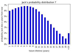
May I introduce you to Jack, an 80 year old American male. According to the United States Life Tables, 2012, he has a remaining life expectancy of 8.3 years. Jack’s future lifetime T is a random variable with a probability distribution shown in the chart below. Some common summary statistics of T are its mean or life expectancy (8.3 years), its median (6.7 years) and its standard deviation (5.1 years).

A (non)linear transformation

Let’s assume that Jack will receive a pension of $20,000 a year. Two transformations on Jack’s future lifetime T are:

(1) $\begin{equation*} V1(T) = \$20,000\;T \end{equation*}$

(2) $\begin{equation*} V2(T) = \$20,000 \frac{(1 + i)}{i} (1 - (1 + i)^{-T}) \end{equation*}$

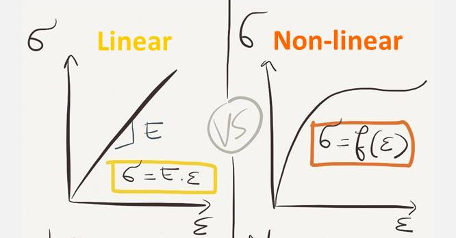
V1(T) reflects the total amount paid to Jack over his remaining lifetime and is a linear function of T.

V2(T) is the present value of these payments for any interest rate i > 0 and is a non-linear function of T.

Both functions are shown in the chart below. For V2(T), we set the discount rate i at 10% to produce a clearly non linear function.

Again, V1(T) and V2(T) are random variables. Performing 100,000 random samples from the probability distribution of T results in the following estimates for the expected value of V1(T) and V2(T):

E[V1(T)] = $166,000
E[V2[T)] = $107,000

At times, it can be tempting to skip the simulation and simply calculate the values of V1 and V2 at the expected future lifetime (=life expectancy):

V1(E[T])] = $166,000
V2[E[T])] = $119,000

As we see, for the linear function V1(T) this approach works fine but once the function becomes non linear like V2(T), we should be careful.

Finally, note that this simple example still allows calculating E[V2(T)] analytically as we have for E[V2(T)] / $20,000:

(3) $\begin{equation*} E[\require{\enclose}\ddot{a}_{\enclose{\actuarial}{T}}] =\sum_{t=0}^{\omega-x}{}_t p_x q_{x+t}\require{\enclose}\ddot{a}_{\enclose{\actuarial}{t+1}} =\sum_{t=0}^{\omega-x} {}_t p_x(1+i)^{-t} \end{equation*}$

where ω = number of rows in the life table.

Conclusion

The average of your simulations can be (roughly) approximated by applying the appropriate transformation on the average of the random inputs. However, take notice this rule of thumb breaks once the relation between the random inputs on one hand and the random outputs on the other hand becomes clearly non-linear.

Deel dit artikel op: