In texts on statistics and machine learning, we often run into the terms standard deviation and standard error. They are both a measure of spread and uncertainty. In this post, we perform three experiments to see how standard deviation and standard error work in practice and how they relate to each other
The formulas I use for the calculations have been summarized in the table at the end of this post. The workbook and data can be found here. In this post, we will define a statistic as a function of observations. Common examples of statistics include the mean, variance, standard deviation, minimum, maximum and percentile of a set of observations.
Experiment #1: throwing a fair die
Throwing a fair die is an experiment with a known uniform distribution. Its population parameters and standard deviation are as follows:
- population mean μ = 3.5
- population variance s^2 = 2.92
- population standard deviation σ = 1.71
These population parameters are known with certainty and therefore do not have a standard error or – as you will – have a standard error equal to zero. From now on, let’s assume we received the following 5 observations not knowing they were generated by throwing a die:
4, 5, 6, 3, 1
Based on this limited amount of information, the best we can do, is calculating estimates for the “real” population values mentioned above. The 5 observations result in the following statistics, each one with its own s.e.:
- sample mean x = 3.8 (s.e. = 0.86)
- sample variance s^2 = 3.7 (s.e. = 1.46)
- sample standard deviation s = 1.92 (s.e. = 0.34)
Looking at the standard errors (s.e.), we immediately see that these statistics are very unreliable estimates for their population counterparts. Let’s do a better job by increasing the sample size from 5 to 30 observations:
4, 5, 6, 3, 1, 6, 1, 6, 3, 4, 4, 6, 1, 3, 6, 4, 4, 3, 5, 4, 2, 1, 5, 5, 3, 3, 5, 5, 1, 1
Based on these 30 observations, we can recalculate the statistics:
- sample mean x = 3.67 (s.e. = 0.32)
- sample variance s^2 = 2.99 (s.e. = 0.51)
- sample standard deviation s = 1.73 (s.e. = 0.13)
Indeed, we see that the statistics are getting closer to their population counterparts while the standard errors are getting closer to 0 (zero). The distributions of the sample mean for samples of size 5 and 30, look as follows:
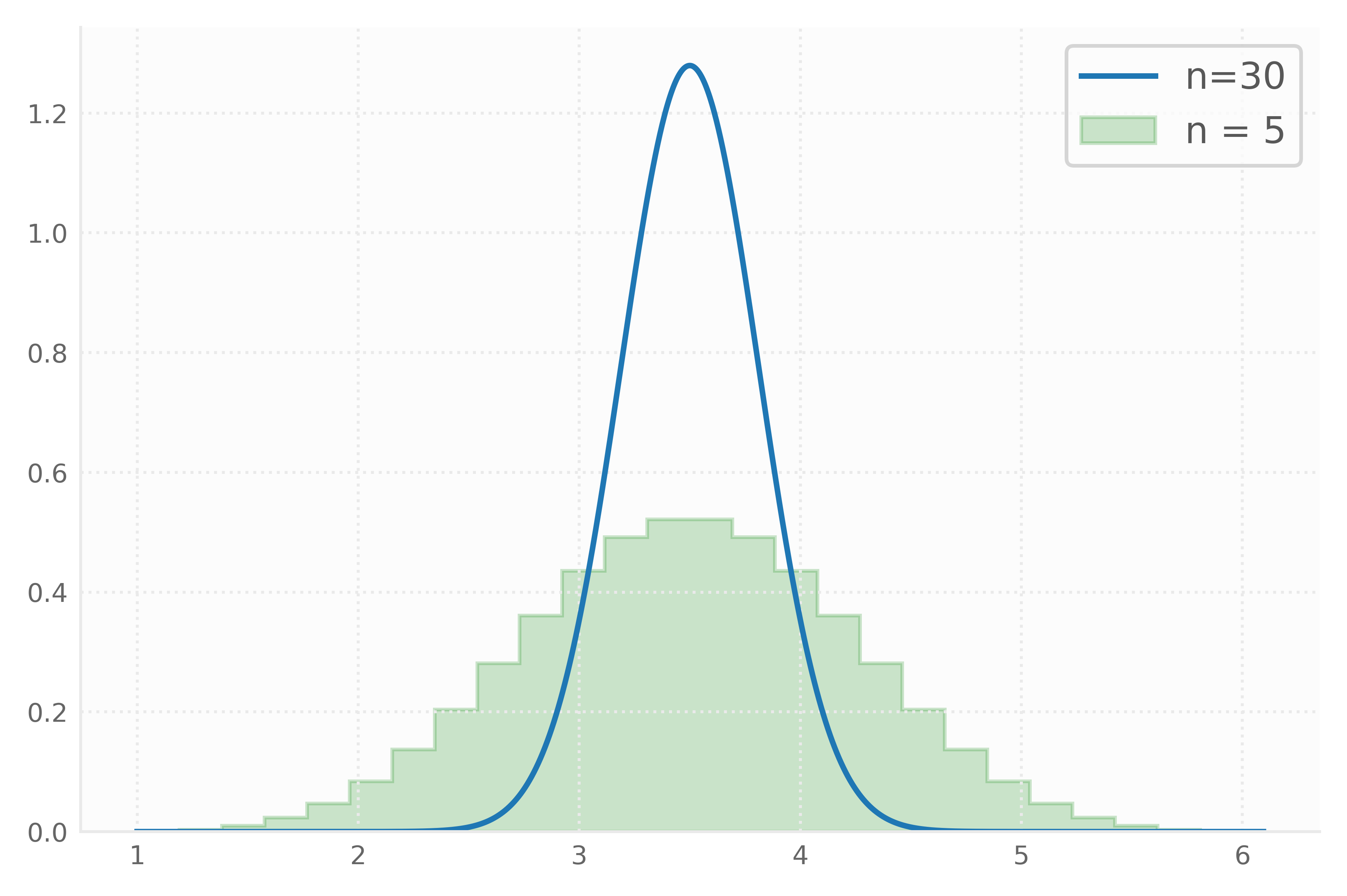
We see that the mean of the distribution tends towards the sample mean (= 3.5) and that the standard deviation gets smaller when the sample size grows larger.
Experiment # 2: simple regression
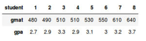
Let’s have a look at the GPA and GMAT scores of the following 8 students:
Performing a simple regression with GPA and GMAT as dependent and independent variables respectively, results in the following statistics, each with its own standard error:
- intercept α = 0.75 (s.e. = 1.96)
- slope β = 0.0043 (s.e. = 0.0013)
- forecasted GPA for a student with GMAT=500: 2.93 (s.e. = 0.21)
- forecast of average GPA for a student with GMAT=500: 2.93 (s.e. = 0.085)
From this we learn that there is a significant relationship between a student’s GPA and his or her GMAT score. In practice, we would refit the model without intercept as this intercept turns out to be insignificant. A student with a GMAT score of 500 is expected to have a GPA of 2.93. Forecasting the GPA of an individual student has more uncertainty than forecasting the average GPA. This is reflected both in the standard errors above and the red and green 95% confidence lines plotted below.
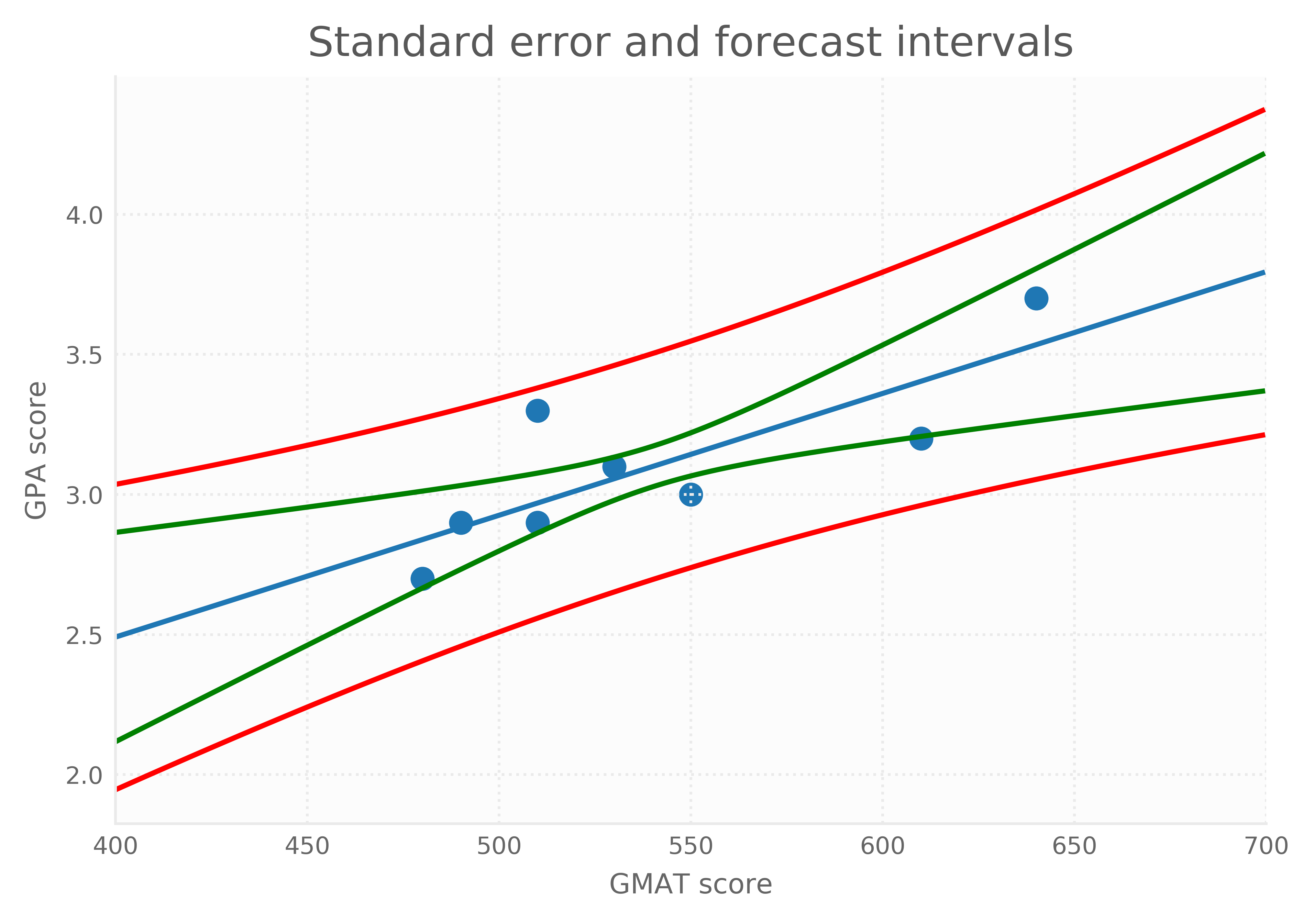
The intervals show that forecasts get more uncertain when we move away from the average score.
Experiment # 3: prostate cancer data
In their book “The Elements of Statistical Learning”, Hastie et all. present the following table, showing the out-of-sample results of several regression models:
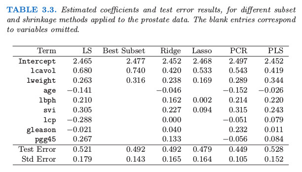
The study was based on 97 patients. The researchers assigned at random 67 patients to the training set and they assigned 30 patients to the test set. How should we read and calculate the numbers in the bottom line of this table, labeled “Std Error”? The numbers turn out to be the standard error of the test error which can be interpreted as a measure of uncertainty when scoring new patients.
Conclusions and suggestions
The standard deviation measures the spread between a set of observations.
The standard error (s.e.) measures the uncertainty of a specific statistic.
As we learned from experiment #1, knowing the exact distribution, result in population statistics like average and standard deviation having standard error 0 (zero). In practice, however, we seldom have the luxury of knowing the exact distribution and we have to draw conclusions based on only a limited number of observations. Based on these observations, a.k.a. a sample, we can calculate several sample statistics, each one with its own standard error.
By increasing the sample size, we can decrease the standard error of a statistic. In other words, the statistic becomes a more reliable estimate for the “real” value as the sample size increases.
As we learned from experiment #2, a regression line can be considered as a statistic with its own standard error. Both its intercept and slope are uncertain. Forecasting new values becomes more uncertain when we move away from the average.
As we learned from experiment #3, the test error is also a statistic with its own standard error.
Actually, the standard error is a statistic having its own standard error. Although not used very often in practice, we could even calculate the standard error of the standard error!
Suggestion #1: when you run into the term standard deviation, ask yourself the following question: does it refer to the “real” standard deviation σσ of the whole population having standard error 0, or does it refer to its estimated counterpart ss having a standard error larger than 0?
Suggestion #2: when you run into the term standard error, ask yourself the following question: what statistic does this standard error belong to?
Last but not least, when calculating any statistic, don’t make any inferences until you have calculated its standard error as it provides you with valuable information about the uncertainty of that statistic!
Appendix: formulas
In case you would like to calculate the numbers mentioned in this post yourself, here are the formulas I used.
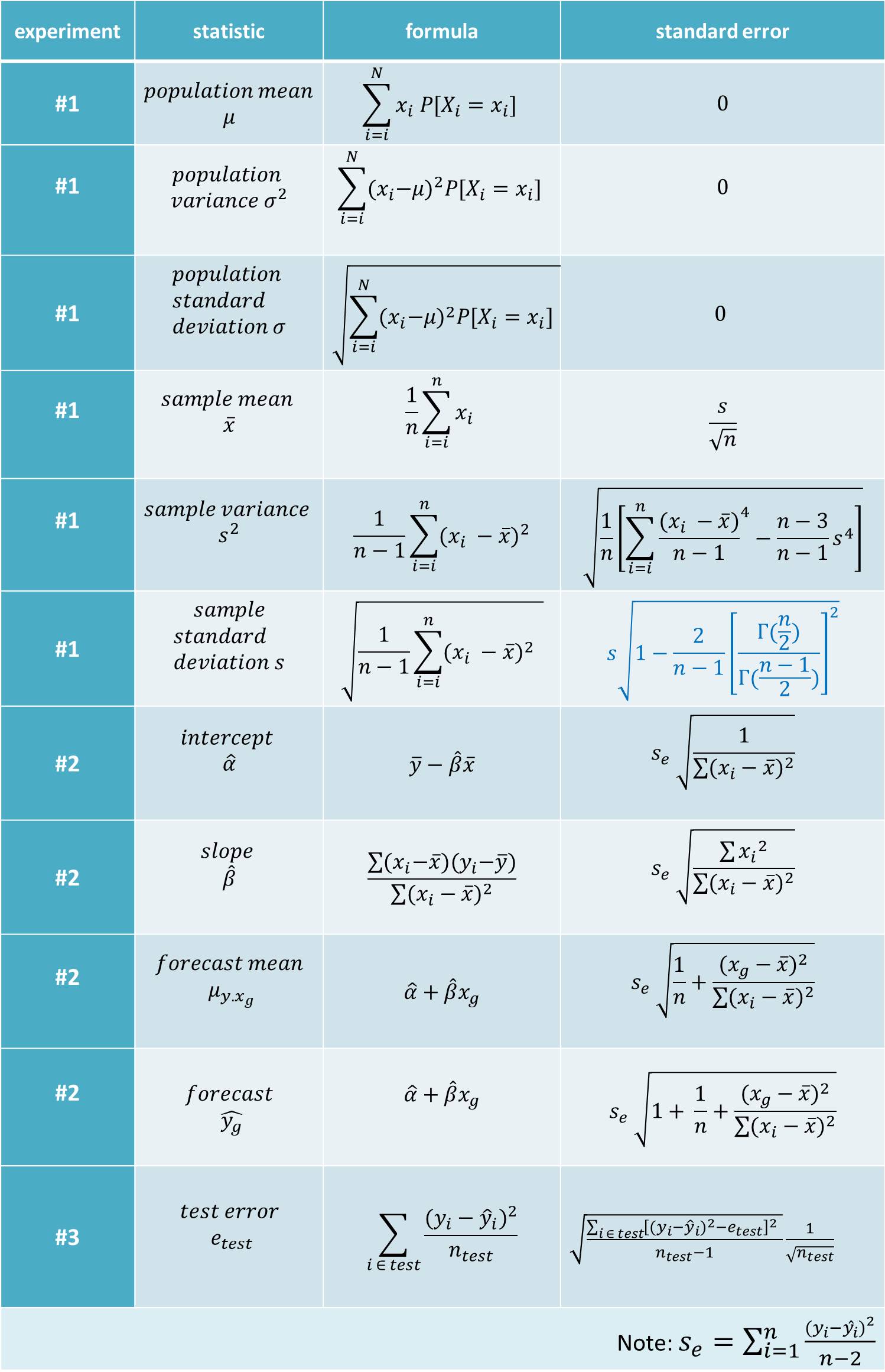
Please note that the formula for the standard error of the standard deviation assumes the observations to come from a normal distribution. In example #1, however, the observations come from a uniform distribution. This is why for calculating the standard error of the standard deviation we did not use the blue formula in the table above, but bootstrapping.