About Backtrader
When it comes to testing and comparing investment strategies, the Python ecosystem offers an interesting alternative for R’s quantstrat. I’m talking here about backtrader, a library that has been around for a while now. Arguably, its object oriented approach offers a more intuitive interface for developing your own strategies than R’s quantstrat. When running the example strategy discussed later on in this post, Backtrader’s default plot facility generates a multi-plot like this:
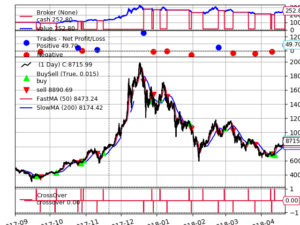
The plot shows time series for 6 months of bitcoin prices, indicators, equity and the entry/exit points of the trades.
Wanted: a Performance Report
In order to make a sound judgment about a specific strategy, I would like to see – on top of the standard plot from Backtrader – a 1 page PDF report featuring both graphical output and performance statistics. The objective of this post is showing how such a performance report may look like.
Installation (local)
$ git clone https://github.com/Oxylo/btreport.git
$ cd btreport
$ pip install -r requirements.txt
Together with a reporting class, these statements will basically install the following dependencies: backtrader, pandas, matpotlib, jinja2 (a templating system for generating HTML documents) and weasyprint (a HTML to PDF converter). The program has been developed and tested on Linux. Windows users have to do some additional work to get the weasyprint library running, see here for instructions.
Approach
I extended Backtrader’s testing engine Cerebro (Spanish for “Brain”) with an additional report method. So, the basic structure for creating the performance report will look like this:
from report import Cerebro

cerebro = Cerebro()

# add your strategy, data, observers, etc here

cerebro.run()
cerebro.plot('output/dir/for/your/report')
Example
As an example, we will have a look at the so called “Golden Cross” strategy on 2018 bitcoin prices (1 hour candles). This strategy entails entering the market if the 50 hour simple moving average (SMA) crosses the 200 hour SMA. Let’s make it a long only strategy, so we close our position if the 50 hour SMA crosses below the 200 hour SMA. When trading in real life, prices can move unexpectedly (slippage!), so it’s a good idea to keep some liquidity on hand at all times. That’s why we invest only 95% of our cash when taking our long position. As a result, our Golden Cross strategy has 3 parameters:
- fast (50 hours)
- slow (200 hours)
- order_pct (95%)
Now it’s time to implement this strategy in Backtrader, as follows:
import os
import sys
import pandas as pd
import backtrader as bt
from report import Cerebro

class CrossOver(bt.Strategy):
    """A simple moving average crossover strategy,
    at SMA 50/200 a.k.a. the "Golden Cross Strategy"
    """
    params = (('fast', 50),
              ('slow', 200),
              ('order_pct', 0.95),
              ('market', 'BTC/USD')
             )

    def __init__(self):
        sma = bt.indicators.SimpleMovingAverage
        cross = bt.indicators.CrossOver
        self.fastma = sma(self.data.close,
                          period=self.p.fast,
                          plotname='FastMA')
        sma = bt.indicators.SimpleMovingAverage
        self.slowma = sma(self.data.close,
                          period=self.p.slow,
                          plotname='SlowMA')
        self.crossover = cross(self.fastma, self.slowma)

    def start(self):
        self.size = None

    def log(self, txt, dt=None):
        """ Logging function for this strategy
        """
        dt = dt or self.datas[0].datetime.date(0)
        time = self.datas[0].datetime.time()
        print('%s - %s, %s' % (dt.isoformat(), time, txt))

    def next(self):
        if self.position.size == 0:
            if self.crossover > 0:
                amount_to_invest = (self.p.order_pct *
                                    self.broker.cash)
                self.size = amount_to_invest / self.data.close
                msg = "*** MKT: {} BUY: {}"
                self.log(msg.format(self.p.market, self.size))
                self.buy(size=self.size)

        if self.position.size > 0:
            # we have an open position or made it to the end of backtest
            last_candle = (self.data.close.buflen() == len(self.data.close) + 1)
            if (self.crossover < 0) or last_candle:
                msg = "*** MKT: {} SELL: {}"
                self.log(msg.format(self.p.market, self.size))
                self.close()
Now we can pour this strategy into the cerebro engine, together with the bitcoin data-feed:
# read the data
TESTDATA = 'btc_usd.csv'
basedir = os.path.abspath(os.path.dirname(__file__))
datadir = os.path.join(basedir, 'sampledata')
infile = os.path.join(datadir, TESTDATA)
ohlc = pd.read_csv(infile, index_col='dt', parse_dates=True)

# initialize the Cerebro engine, now extended with a report method
cerebro = Cerebro()
cerebro.broker.setcash(100)

# add data
feed = bt.feeds.PandasData(dataname=ohlc)
cerebro.adddata(feed)

# add Golden Cross strategy
params = (('fast', 50),
          ('slow', 200),
          ('order_pct', 0.95),
          ('market', 'BTC/USD')
          )
cerebro.addstrategy(strategy=CrossOver, **dict(params))
Finally, we run the backtest and generate the report:
cerebro.run()
cerebro.report('output/dir/for/your/report')
This should be enough to generate the performance report. If you would like to enrich the report with some additional descriptives like details about your data-feed, your user name and/or comments, you can pass this to the report method:
cerebro.report('output/dir/for/report',
               infile='btc_usd.csv',
               user='Trading John',
               memo='Golden Cross / BTC')
Output
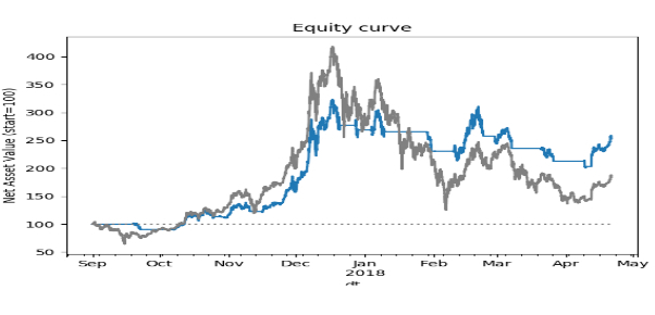
After running the strategy described above, the 1 page PDF performance report (in JPG here for convenience) looks as follows:
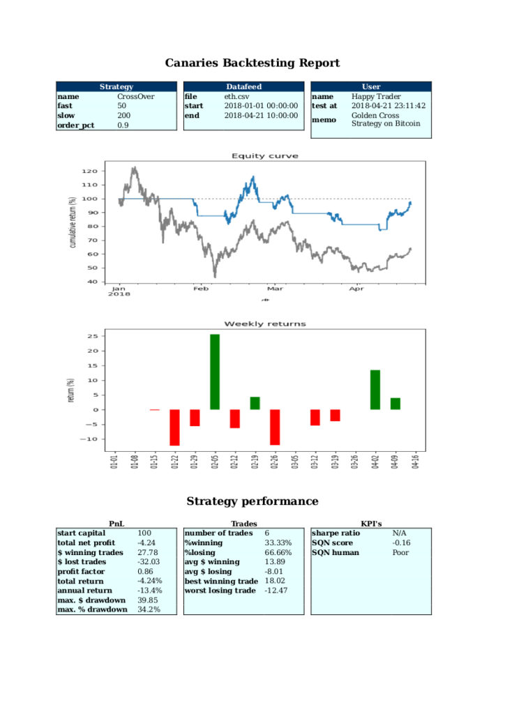
When investing in bitcoin, you should be prepared for a rough ride, as shown by the grey line in the Equity curve plot (“Buy & Hold”). The last months of 2017 were extremely bullish till around Christmas when the sentiment turned bearish due to (proposed) bans in Asia (among others). The blue line in in the Equity curve plot shows how equity would have developed if the Golden Cross strategy, as described above, had been applied. Over the last 6 months, the Golden Cross strategy (blue) clearly beats Buy & Hold (grey) but the favorable returns (152% over 6 months time) come at the price of high risk as shown by the Sharpe ratio of only 0.57.
Acknowledgements: I would like to express my gratitude to the following amazing individuals for their contributions and suggestions: James Campell (algotrading in general), Chris Moffitt (for his excellent post on generating PDF with Python) and my partners in crime in what we have called the canaries project: Erwin Bakker, Eddy Chan and Michael van der Waeter.