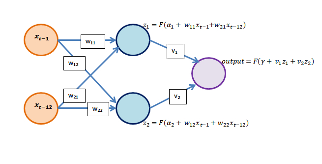
In this post, we will build an autoregressive neural network using a few lines of R code.
Gas consumption
A couple of weeks ago I started working on data for a large energy provider in the Netherlands. Being a newbie in this sector, one of my first actions was having a serious look at our household's energy bill. Fortunately, my wife has always been an excellent bookkeeper and she had kept meticulously track of our monthly gas consumption:
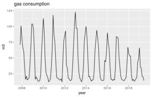
We use gas for cooking, when taking a warm shower and for heating the house. Therefore, it's little surprising that gas consumption is high in winter and low in summer and there is a clear pattern visible in the graph. I was wondering how a neural network would perform when it comes to recognizing this pattern.
Training a neural net and performing forecasts
Let's do some coding:
library(forecast)
data = read.csv('eneco.data')
myts = ts(data$gas, start=c(2007, 11), end=c(2019, 6), frequency=12)
ann = nnetar(myts, lambda=0)
fc = forecast(ann, h=12)
autoplot(fc, main='gas consumption', xlab='year', ylab='m3')
This results in the following plot where the blue curve shows the 12 months prediction:
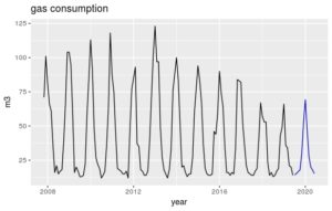
In case you would like to reproduce this result, you can find the code and the data here
What happens in the rest of the code? In line 3, the data frame is converted to a time series. This is not strictly required but comes in handy when plotting the series with nice ticks on the x-axis. Line 4 is where the magic happens. The nnetar() function fits an NNAR(p,P,k)[m] model ("Neural Net Auto Regressive") with the following parameters:
- p = number of non-seasonal lags as inputs
- P = number of seasonal lags as inputs
- k = number of hidden nodes in the hidden layer
- m = frequency of the data
As p, P and k are not specified in our nnetar() function, they are selected automatically. By default, k equals the number of input nodes + 1, rounded up to the nearest integer. To make sure that the forecasts for the gas consumption stay positive, we included a Box-Cox transformation with lambda=0. Line 5 creates a forecast object resulting in a prediction for the next 12 months. Line 6, finally, plots this object with an appropriate labeling for the axes. For our data, nnetar() found a neural net with p=1, P=1, k=2 and m=12. In other words, the model takes as inputs the gas consumption at t-1 and t-12 and has one hidden layer with 2 neurons as shown in the figure below.
As shown in the picture, training the neural network entails estimating 9 different parameters, 3 for each neuron in the hidden layer and output layer.
Prediction intervals
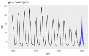
Unlike linear regression, neural networks do not have a closed expression for the uncertainty margin around the predictions. However, nnetar() has a PI parameters which allows simulating several (by default 1,000) future sample paths for the gas consumption data:
fc = forecast(ann, PI=TRUE, h=12)
autoplot(fc, main='gas consumption', xlab='year', ylab='m3')
This results in the following plot with prediction intervals around the forecasts:
Walk forward analysis
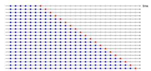
How well does the neural network perform when it comes to making one-month-ahead predictions for the gas consumption? Performing a walk forward analysis entails training the model on past observations (blue dots) to predict the next observation (red dot). This procedure is repeated using a rolling window, as illustrated in the picture below (thanks to Rob Hyndman, author of the forecast package).
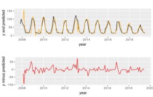
The result of the walk forward analysis has been summarized in the picture below. The black line represents the actual observations; the orange line represents the one-month-ahead predictions. The error, simply the difference between the black line and the orange line, is represented by the red line.
Conclusion
The forecast library in R offers a compact and well-documented tool for building, among others, autoregressive neural networks in just a few lines of code. Support for creating prediction intervals and walk forward analysis gives insight into the predictive power of the neural network.

